EVIDENCE BASED MEDICINE SERIES

Pdf version

Part 3. APPRAISING THE EVIDENCE
Results: Clinically Important?

Next, we go through the concept of specificity by looking at the other half of the table.

Table 3. The “right-half” of Table 1, used for illustrating the concept of specificity

	Not diseased
Test result positive	c
Test result negative	d

Here, we can see that we only deal with patients without the disease. The total number of patients without the disease is represented by the whole column, the sum of c and d. The upper cell, c, is the number of patients without the disease, in whom the test shows up (“incorrectly”) as positive. The lower cell, d, is the number of patients without the disease, in whom the test shows up (“correctly”) as negative.

Specificity is represented by the formula: d/c+d. In words, it is the percentage of people without the disease that are correctly identified by the test. The higher is the specificity, the smaller is c, which means fewer disease-free persons would be tested positive, and get a false alarm. 

The concept of sensitivity and specificity is useful when we assess patients at the bedside, thinking through their likelihood of having the disease from our clinical assessment, and pondering on the added value of a diagnostic test in helping us make our diagnosis. A diagnostic tool with high sensitivity is necessary in primary setting where screening takes place, and where we refer patients who are suspected to have the disease for further work-up. On the other hand, a tool with high specificity is preferable in tertiary centres where patients have already undergone some form of prior assessments, to avoid unduly labeling healthy people as diseased and subject them to unnecessary anxiety, and even treatment.  In general, for both sensitivity and specificity, figures above 80% are taken as acceptable, and above 90% as excellent. 

Predictive values

Once a diagnostic test is ordered and the results available, the concepts of sensitivity and specificity are no longer directly applicable. Instead, we look to see how accurate the available results of the test are in predicting the likelihood of having the disease. These measures are called predictive values. There are two types of predictive value, namely positive and negative predictive values. Let us explore each of these terms using again, parts of Table 1.

Table 4. The “top-half” of Table 1, used for illustrating the concept of positive predictive value

	Diseased	Not diseased
Test result positive	a	c

In dealing with sensitivity and specificity, we look down the columns. In dealing with predictive values, we look across the rows. Shown here is the upper row of the table, where everyone has a positive test result, while some truly have the disease (a), and some do not have the disease (c).

Positive predictive value of a test, represented by the formula a/a+c, is the proportion of those with positive test result who truly have the disease.

Table 5. The “bottom-half” of Table 1, used for illustrating the concept of negative predictive value

	Diseased	Not diseased
Test result negative	b	d

Similarly, looking at Table 5, negative predictive value, represented by the formula d/b+d, is the proportion of those with negative test result who truly do not have the disease. 

Likelihood ratios

Compared to earlier terms, likelihood ratios are less intuitive, but probably more complete measures of the performance of a diagnostic test. From the notes above, one may notice that sensitivity, specificity and predictive values, if considered alone, tell us only part of the story about a diagnostic test (only parts of the 2x2 table is used when illustrating each of these terms). In likelihood ratios, we combine both sensitivity and specificity into a single measure.

There are two types of likelihood ratio – the likelihood ratio for a positive result (LR+) and the likelihood ration for a negative result (LR -).

LR+ is represented by the formula: Sensitivity/(1-specificity). It tells us how much the odds of the disease increases when the test is positive.

LR- is represented by the formula: (1-sensitivity)/specificity. It tells us how much the odds of the disease decreases when the test is negative.

The odds of a disease is the ratio between the number who have the disease over the number who do not have the disease.  This is different from the usual terms of “risk” or “probability”, in which the denominator is the total number of patients. Although less intuitive, measures involving odds are widely used for different reasons, the details of which are beyond the scope of this article. 

STUDIES ON PROGNOSIS

In a study on prognosis, the authors look at the association between a factor, called the prognostic indicator, and the outcome. For example, patients with “stage 2BX, high grade” Non-Hodgkins Lymphoma (NHL) (prognostic indicator) and five-year disease-free survival (outcome). Among the three major elements that determine the clinical importance of such studies, clinical relevance of the outcome is straightforward, and the precision of the estimates is covered in the previous section on therapy. We shall now focus on the remaining element: the comprehensiveness of the information relating to the outcome over time.

Take the example above on NHL and survival. Let’s say the study finds that the five-year disease-free survival rate for patients with such specific staging and grading of NHL is 50%. We know that at the end of the five-year period 50% of the patients survive. That is all we know. But surely, we and our patients would be interested to find out what happens along the five years. We may ask: among the 50% who did not survive, was there a steady increase in mortality over the years of follow-up? When did most of this 50% of patients die?  Between the fourth and fifth year, or during the first year?.... These are crucial information for our patients and their family, who may well be planning their future.

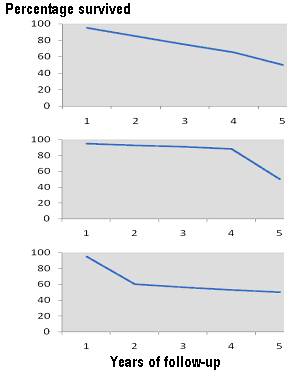
A study on prognosis provides clinically useful and important results by providing us the information on the likelihood of the outcome over time. This is often best demonstrated using graphs called the survival curves (see Figure 1). The curves are commonly used to depict all outcomes over time in general, not only survival.

Figure 1. Three survival curves, each showing a five-year survival rate of 50% but different trends of survival over the five years

The three graphs contained in Figure 1 all end up with 50% survival rate at the end of the five-year period, but each has different trend of survival over time. The top graph shows a steady decrease in survival rate over the five years, the middle shows a minimal decrease in the first four years followed by a sharp drop between the fourth and the fifth year, while the bottom graph shows a sharp decrease over the first year and a slow drop thereafter. It should be self-evident that such information is critical in counselling patients about their prognosis. 

Summary

It may be obvious to the readers now that critical appraisal, especially evaluating the clinical importance of evidence, is not a robotic process. Apart from understanding the various means of expressing a study result, it takes into account factors other than the evidence itself, like the clinical circumstances and the individual judgment of the clinicians who make decisions on whether the treatment, diagnostic tool or prognostic information is worth using in practice.

REFERENCES

1. Altman DG. The scandal of poor medical research. BMJ. 1994;308(6924):283-4 [PubMed] [Full text]
2. Straus SE, Richardson WS, Glasziou P, Haynes RB. Evidence-based medicine. How to practice and teach EBM. 3rd ed.: Edinburgh: Churchill Livingstone; 2005.
3. Teaching EBM: Teaching materials: Critical appraisal worksheets.  Toronto: Centre for Evidence Based Medicine: University Health Network. Available from: http://www.cebm.utoronto.ca/teach/materials/caworksheets.htm
4. Appraising.  Available from: http://www.shef.ac.uk/scharr/ir/netting/
5. Critical appraisal. Available from: http://www.cebm.net/index.aspx?o=1157.
6. Evidence-Based Medicine for Primary Care and Internal Medicine. BMJ Publishing Group; 2009. Available from: http://ebm.bmj.com
7. Glasziou P, Del Mar C, Salisbury J. Evidence-based practice workbook: bridging the gap between health care research and practice. Wiley-Blackwell; 2007
8. Dans A, Dans L, Silvestre M. Painless Evidence-Based Medicine. Chichester: John Wiley and Sons Ltd; 2007
9. Edwards A, Elwyn G, Mulley A. Explaining risks: turning numerical data into meaningful pictures. BMJ. 2002;324(7341):827- 30 [PubMed] [Full text]